


New in DAX: Window Functions!
Microsoft presented ‘new good stuff’ again in the December release of Power BI desktop. There are three (3) new Dax functions we can enjoy: OFFSET, INDEX and WINDOW. These are so called “window” functions, related to SQL Window functions we know in SQL.
So what is a window function? This function will do a calculation across a set of table rows, that are connected to the current row. This means that these functions help you to compare the current row to the previous row, do a calculation across multiple rows like for example a running total. But let’s not dwell on the definition and have a look at some examples where these functions can do some good and help you in with calculations in your reports.
The Demo Data
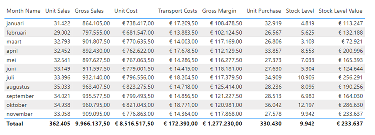
To explain the use of the 3 new DAX functions I use a dataset of six stores that sell pizzas. The overview below shows of their sales, margin and stock numbers.
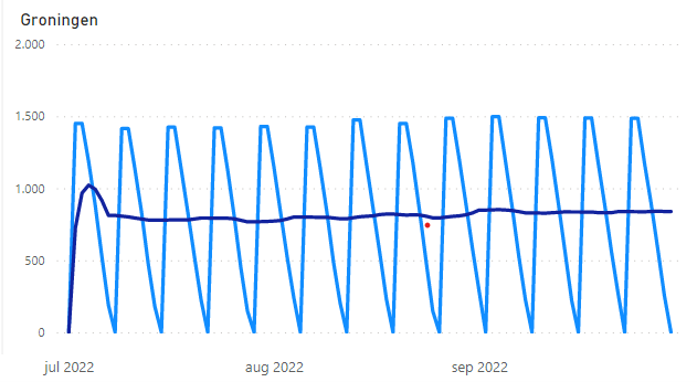
Every Saturday the stores receive a new delivery of stock items, on Sunday they are closed and the other days they sell their pizzas. Looking at the stock of one of the stores you can see very clearly the weekly cycle of receiving the products on Saturday and selling it up until the next Saturday.

As Groningen’s stock hits 0 each time, it might be smart to have a bit more stock, but that’s something the business can take care of 😊
INDEX
First of all let’s look at the function INDEX: INDEX points to an absolute position in the table. If you count 1,2,3 you are counting from the top of the table, with -1,-2,-3 you count from the bottom of the table.
INDEX ( <position>[, <relation>][, <orderBy>][, <blanks>][, <partitionBy>] )
This function is very useful if you want the last or the first row of a period. Additionally if you sort your customers by Sales, you can get the Top and bottom customers by using this function. In the example below we use the INDEX function to get the stock at the beginning and at the end of the month.
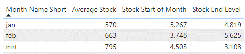
You see that the average stock is much lower than the start- and end level. As the start- and end days were close after the delivery of new product so at that point there was a lot of stock. To do the calculation of Start of month and End of month I used this DAX expression.
Stock End Level =
VAR _table =
SUMMARIZE (
ALL ( ‘Stock’ ),
Stores[Store Name],
‘Date'[Month Name Short],
‘Date'[Date]
)
RETURN
CALCULATE (
[Stock Level],
INDEX (
-1,
_table,
ORDERBY ( ‘Date'[Date] ),
KEEP,
PARTITIONBY ( Stores[Store Name], ‘Date'[Month Name Short] )
)
)
A few points to clarify:
- You see the -1, that number points to the first row counted from the bottom of the table.
- The variable _table shows the table itself, being the stock data with store name and date.
- The third thing to notice is PARTITIONBY. this parameter partitions the table, in this case it partitions the table into Store and Month so that for each Store and Month we have a separate partition where the count starts and stops. This makes sense as you don’t want to mix numbers for different months or stores in your month end number, so it enables index to point at the last number for this month and this store.
- Finally, notice that I used the original measure [Stock Level], that is the same measure I used for Average Stock in the other column. The difference being that I get the stock level from another place in the table.
OFFSET
The second function in the windows functions is OFFSET. The difference to the previous INDEX function is that offset is relative to the current line. So, if you use OFFSET -1 on a table based on date, the offset function will look at the day before the current row. Technically you can do some tricks to count rows and use INDEX but OFFSET is much easier.
OFFSET ( <delta>[, <relation>][, <orderBy>][, <blanks>][, <partitionBy>] )
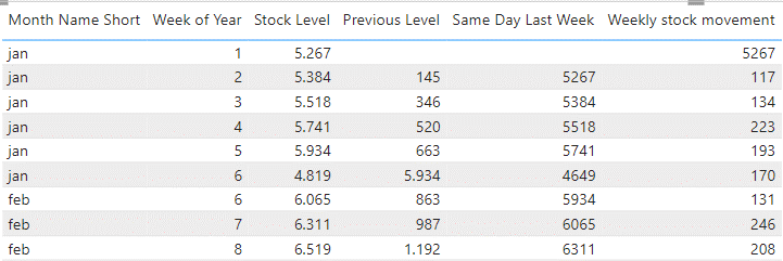
To demonstrate the use of the OFFSET I look at the stock in de table below and I want to see how much it changed since last week. You can see it looks at the same day last week (in our sample important, because Saturday is delivery day) and it looks at the movement.
The DAX expression I used:
Same Day Last Week =
VAR _table =
SUMMARIZE (
ALL ( ‘Stock’ ),
Stores[Store Name],
‘Date'[Date]
)
RETURN
CALCULATE (
[Stock Level],
OFFSET (
-7,
_table,
ORDERBY ( ‘Date'[Date] ),
KEEP,
PARTITIONBY ( Stores[Store Name] )
)
)
You see the same items appear as in INDEX, but now Offset points to -7, so 7 rows before. Because I have all the dates, that means same weekday, a week earlier.
WINDOW
The last function is WINDOW. The difference to INDEX and OFFSET is that this function has a start and an endpoint. So you can pick up multiple rows with this function. You can set the start- and endpoint as Relative (REL) or Absolute(ABS).
WINDOW ( from[, from_type], to[, to_type][, <relation>][, <orderBy>][, <blanks>][, <partitionBy>] )
In our example we use the WINDOW function to create a rolling average for the week as that takes care of the cycle of purchasing and selling which makes the graph look less like saw teeth.
I use WINDOWS with relative positions like –6, REL, 0, REL, to create the rolling average. The DAX expression I defined:
Rolling Average 7 days =
VAR _Table =
SUMMARIZE (
ALLSELECTED ( ‘Stock’ ),
Stores[Store Name],
‘Date'[Date]
)
RETURN
CALCULATE (
[Average Stock],
WINDOW (
-6,
REL,
0,
REL,
_table,
ORDERBY ( ‘Date'[Date] ),
KEEP,
PARTITIONBY ( Stores[Store Name] )
)
)
Another way to use WINDOW is for Year to Date. If you partition by Year , use position 1, ABS and 0, REL you will get every row from the start of the year until the current day.
Summary
In this blog I explained how you can use OFFSET, INDEX and WINDOW to do cross-row calculations. INDEX can be used to get a row based on the absolute row count. OFFSET can be used to get a row relative to the current row. And WINDOW is a Swiss army knife that can do both and additionally use multiple rows.
In the future these functions will be developed further. You can find an overview of all the DAX filter functions here. If you want to do a deep-dive, I can recommend the following articles from one of the Power BI developers:
The Power BI developers warn that these functions still have some limitations and issues. But my advice is to try these functions just to see what it can do. Meanwhile the DAX product team will be busy on improvements and new features.